


In a separate blog post, we have discussed the problem of outlier detection using statistical tests. Generally speaking, statistical tests are suitable for detecting outliers that have extreme values in some numerical features. However, outliers are many and varied, and not all kind of outliers can be characterized by extreme values. In many cases for outlier detection, statistical tests become insufficient, or even inapplicable at all.
In this blog post, we will use a clustering algorithm provided by SAP HANA Predictive Analysis Library(PAL) and wrapped up in the Python machine learning client for SAP HANA(hana_ml) for outlier detection. The algorithm is called density-based spatial clustering of applications with noise, or DBSCAN for short. Basically, you will learn:
- The mechanism of DBSCAN for differentiating outliers from inliers
- How to apply the DBSCAN algorithms in hana_ml and extract the information of detected outliers
Introduction

Solutions
For better illustration, in the following context we use DBSCAN to detect outliers in two datasets: one is a mocking dataset that has been depicted in the introduction section, another is the renowned iris dataset.
Connect to HANA
import hana_ml

from hana_ml.dataframe import ConnectionContext

cc = ConnectionContext(address='xxx.xxx.xxx.xxx', port=30x15, user='XXXXXX', password='XXXXXX')#account details omitted
Use Case I : Outlier Detection with Mocking Data
The mocking data is stored in database in a table with name 'PAL_MOCKING_DBSCAN_DATA_TBL', we can use the table() function of ConnectionContext to create a corresponding hana_ml.DataFrame object for it.
mocking_df = cc.table('PAL_MOCKING_DBSCAN_DATA_TBL')The collect() function of hana_ml.DataFrame can help to fetch data from database to the python client, illustrated as follows:
mocking_df.collect()

The record with ID 800 corresponds to the purple point in the graph as shown in the introduction section.
Next we import the DBSCAN algorithm from hana_ml, and apply it to the mocking dataset.
from hana_ml.algorithms.pal.clustering import DBSCAN

dbscan = DBSCAN(minpts=4, eps=0.2)#minpts and eps are heuristically determined

res_mock = dbscan.fit_predict(data=mocking_df, key='ID', features=['X', 'Y'])#select numerical features only

res_mock.collect()

In the result table of DBSCAN, most records are assigned with their corresponding non-negative cluster IDs, while detected outliers are commonly assigned with cluster ID -1. Direct view of the result confirms that the centered outlier has been successfully detected as our expectation. We can refer to the 'CLUSTER_ID' column of the clustering result table to check whether other points have been detected as outliers, which is illustrated as follows:
outlier_ids = cc.sql('SELECT ID FROM ({}) WHERE CLUSTER_ID = -1'.format(res_mock.select_statement))
outlier_ids.collect() So the centered point is the single detected outlier, which is consistent with our visual perception of the data .
Use Case II : Outlier Detection with IRIS Dataset
iris_df  = cc.table('PAL_IRIS_DATA_TBL')

iris_df.collect()
Now we apply DBSCAN algorithm to the iris dataset for outlier detection, illustrated as follows:
from hana_ml.algorithms.pal.clustering import DBSCAN

dbscan = DBSCAN(minpts=4, eps=0.6)#minpts and eps are heuristically determined

res_iris = dbscan.fit_predict(data=iris_df, key='ID',

                         features=['SepalLengthCm',

                                   'SepalWidthCm',

                                   'PetalLengthCm',

                                   'PetalWidthCm'])#select numerical features only

res_iris.collect()
As shown by the clustering result, the algorithm separates the inliers of the iris dataset into 2 clusters, labeled with 0 and 1 respectively. Outliers are also detected, illustrated as follows:

In the following context we try to visualize the clustering result, so as to making sure that outliers are appropriately detected.
We first partition the clustering result based on assigned cluster IDs.
cluster0 = cc.sql('SELECT * FROM ({}) WHERE CLUSTER_ID = 0'.format(res.select_statement))

cluster1 = cc.sql('SELECT * FROM ({}) WHERE CLUSTER_ID = 1'.format(res.select_statement))
Now each part contains the original data IDs so that we can perform select operation from the original dataset. However, points selected from original dataset is naturally 4D and thus could not be visualized by regular 2D/3D plots. We can use dimensionality techniques to overcome this difficulty. In the following content we use principal component analysis(PCA) for dimensionality reduction.
from hana_ml.algorithms.pal.decomposition import PCA

pca = PCA()

iris_dt = pca.fit_transform(data = iris_df,

                            key = 'ID',

                            features=['SepalLengthCm',

                                      'SepalWidthCm',

                                      'PetalLengthCm',

                                      'PetalWidthCm'])

iris_2d = iris_dt[['ID', 'COMPONENT_1', 'COMPONENT_2']]

iris_2d.collect()
The dataset has been transformed from 4D to 2D, we can select transformed data points from transformed data w.r.t. the assigned cluster labels.
outlier_2d =  cc.sql('select * from ({}) where ID in (select ID from ({}))'.format(iris_2d.select_statement,

              outlier.select_statement))

cluster0_2d = cc.sql('select * from ({}) where ID in (select ID from ({}))'.format(iris_2d.select_statement,

              cluster0.select_statement))

cluster1_2d = cc.sql('select * from ({}) where ID in (select ID from ({}))'.format(iris_2d.select_statement,

              cluster1.select_statement))
Now we can visualize the outlier detection result on the dimensionality reduced dataset.
import matplotlib.pyplot as plt

plt.scatter(x = cluster0_2d.collect()['COMPONENT_1'],

            y = cluster0_2d.collect()['COMPONENT_2'],

            c='brown')

plt.scatter(x = cluster1_2d.collect()['COMPONENT_1'],

            y = cluster1_2d.collect()['COMPONENT_2'],

            c='red')

plt.scatter(x = outlier_2d.collect()['COMPONENT_1'],

            y = outlier_2d.collect()['COMPONENT_2'],

            c='green')

plt.legend(['Cluster 0', 'Cluster 1', 'Outliers'])

plt.show()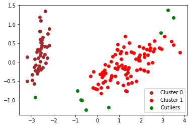
Detected outliers are marked by green dots in the above figure. We see that most marked outliers are isolated other regularly clustered points in the transformed space, so the detection result makes sense in general.
Discussion and Summary
 Bluesky


You must be a registered user to add a comment. If you've already registered, sign in. Otherwise, register and sign in.