
-
Products and Technology
By Category
-
Groups
Activity Groups
Industry Groups
Influence and Feedback Groups
Interest Groups
Location Groups
Customer Only Groups
- Developers
- Partners
- Events
- Help Center
- Topic Pages
-
Explore SAP
Products
- Autonomous Enterprise
- Artificial intelligence
- Data and analytics
- Autonomous Suite
- Technology platform
- Transformation management
- Midsize business solutions
- Financial management
- Spend management
- Supply chain management
- Human capital management
- Customer experience
- Enterprise resource planning
- Business network
- Sustainability management
- SAP Store
- Try SAP
- View all industries
- Partners
- Services
Learning and Support
-
- Products and Technology
- Groups
- Developers
- Partners
- Events
- Help Center
- Topic Pages
-
Explore SAP
- Explore SAP
-
Products
- Products
- Autonomous Enterprise
- Artificial intelligence
- Data and analytics
- Autonomous Suite
- Technology platform
- Transformation management
- Midsize business solutions
- Financial management
- Spend management
- Supply chain management
- Human capital management
- Customer experience
- Enterprise resource planning
- Business network
- Sustainability management
- SAP Store
- Try SAP
- View all industries
- Partners
- Services
- Learning and Support
- About
- SAP Community
- Products and Technology
- Technology
- Technology Blog Posts by SAP
- A Multivariate Time Series Modeling and Forecastin...
- Subscribe to RSS Feed
- Mark as New
- Mark as Read
- Bookmark
- Subscribe
- Printer Friendly Page
- Report Inappropriate Content
- SAP Managed Tags
- Machine Learning
- SAP HANA Cloud
- Python
- SQL
- SAP HANA
- Big Data
Picture this: you are the manager of a supermarket and want to forecast sales for the next few weeks based on historical daily sales data for hundreds of products. What kind of problem would you classify this as? Naturally, time series modeling methods such as ARIMA and exponential smoothing may come to mind first. With these tools, you could treat the sales of each product as a separate time series and predict future sales based on historical values.
After a moment, you realize that the sales of these products are not independent and that there are dependencies among them. For example, during festivals, the promotion of barbecue meat may also boost sales of ketchup and other spices. If one brand of toothpaste is on sale, demand for other brands might decline. These kinds of relationships are common. When multiple variables interact, we need a suitable tool for multivariate time series (MTS) analysis that can capture dependencies between variables.
In SAP HANA Predictive Analysis Library (PAL), wrapped in the Python Machine Learning Client for SAP HANA (hana-ml), one of the most commonly used and powerful methods for MTS forecasting is VectorARIMA, which includes several model types such as VAR, VARX, VMA, VARMA, and VARMAX.
In this blog post, you will learn:
- An introduction to MTS and VectorARIMA.
- A use case that walks through the main steps of VectorARIMA implementation.
This blog post assumes that you already have some familiarity with univariate time series and ARIMA modeling (AR, MA, ARIMAX, sARIMA, …). In hana-ml, we also provide tools such as ARIMA and AutoARIMA, and you can refer to the documentation for further information.
1. Introduction to MTS and VectorARIMA
A multivariate time series consists of more than one time-dependent variable, and each variable depends not only on its own past values but also on other variables.
One of the most popular methods for handling MTS is the Vector Autoregressive Moving Average (VARMA) model, which is a multivariate extension of autoregressive integrated moving average (ARIMA) and can be used to examine relationships among several variables.
In hana-ml, the VARMA-related function is called VectorARIMA, which supports a range of model types, including pure VAR, pure VMA, VARX (VAR with exogenous variables), seasonal VARMA, and VARMAX. Similar to ARIMA, building a VectorARIMA model requires selecting the appropriate autoregressive order p, moving-average order q, and differencing degree d. If seasonality exists in the time series, seasonal parameters must also be specified, including seasonal period s, vector seasonal AR order P, vector seasonal MA order Q, and seasonal differencing degree D.
In VectorARIMA, the orders of VAR, VMA, and VARMA models can be specified automatically. Note that the degree of differencing must be provided by the user and is determined by making the time series stationary.
In the auto selection of p and q, there are two search options for VARMA model: performing grid search to minimize some information criteria (also applied for seasonal data), or computing the p-value table of the extended cross-correlation matrices (eccm) and comparing its elements with the type I error. VAR model uses grid search to specify orders while VMA model performs multivariate Ljung-Box tests to specify orders.
2. Solutions
In this section, a use case is presented to walk through the main steps of VectorARIMA implementation.
2.1 Dataset
A public dataset in Yash P Mehra’s 1994 article: “Wage Growth and the Inflation Process: An Empirical Approach” is used and all data is quarterly and covers the period 1959Q1 to 1988Q4. The dataset has 123 rows and 8 columns and the definition of columns are shown below.
- rgnp : Real GNP.
- pgnp : Potential real GNP.
- ulc : Unit labor cost.
- gdfco : Fixed weight deflator for personal consumption expenditure excluding food and energy.
- gdf : Fixed weight GNP deflator.
- gdfim : Fixed weight import deflator.
- gdfcf : Fixed weight deflator for food in personal consumption expenditure.
- gdfce : Fixed weight deflator for energy in personal consumption expenditure.
The dataset can be downloaded here.
The figure below visualizes the data. From inspection, none of the eight variables shows obvious seasonality, and each curve trends upward. Therefore, in the following analysis, we do not consider seasonality in the model.

Fig. 1. Curves of 8 variables
The source code uses the Python Machine Learning Client for SAP HANA.
2.2 SAP HANA Connection
The first step is to establish a connection to SAP HANA. Once the connection context is created, we can use various hana-ml functions to analyze the data. The following script is an example:
import hana_ml
from hana_ml import dataframe
conn = dataframe.ConnectionContext(address='AAA.BBB.CCC.DDD', port=XXX, user='username', password='password')
Replace ‘AAA.BBB.CCC.DDD’, ‘XXX’, ‘username’, and ‘password’ with your SAP HANA instance details.
2.3 Data Splitting
The dataset has been imported into SAP HANA with the table name “GNP_DATA”. Therefore, we can access the table via the dataframe.ConnectionContext.table() function. We then add a column called ‘ID’ to the original DataFrame df because VectorARIMA() requires an integer key column. Next, we select the first 80% of df (99 rows) as training data and the remaining 20% (24 rows) as test data for the next step.
# The 'date' column in the original csv file has been dropped
df = conn.table('GNP_DATA')
# Add a ID column
df = df.add_id('ID')
# select 80% of data as the training data and the rest as the test data
df_train = df.filter('ID <= 99')
df_test = df.filter('ID > 99')
print(df_train.head(5).collect())
print(df_test.head(5).collect()) 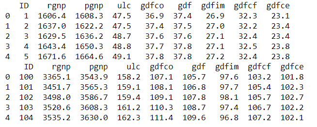
2.4 Model Building
The data is ready, let's start the trip of MTS modeling! We will involve the steps below:
- Causality investigation
- Test for stationary
- Model Building
- Test for residuals (errors)
2.4.1 Causality Investigation
First, we use Granger Causality Test to investigate causality of data. Granger causality is a way to investigate the causality between two variables in a time series which actually means if a particular variable comes before another in the time series. In the MTS, we will test the causality of all combinations of pairs of variables.
The Null Hypothesis of the Granger Causality Test is that lagged x-values do not explain the variation in y, so the x does not cause y. We use grangercausalitytests function in the package statsmodels to do the test and the output of the matrix is the minimum p-value when computes the test for all lags up to maxlag. The critical value we use is 5% and if the p-value of a pair of variables is smaller than 0.05, we could say with 95% confidence that a predictor x causes a response y.
The script is below:
from statsmodels.tsa.stattools import grangercausalitytests
variables=data.columns
matrix = pd.DataFrame(np.zeros((len(variables), len(variables))), columns=variables, index=variables)
for col in matrix.columns:
    for row in matrix.index:
        test_result = grangercausalitytests(data[[row, col]], maxlag=20, verbose=False)
        p_values = [round(test_result[i+1][0]['ssr_chi2test'][1],4) for i in range(maxlag)]
        min_p_value = np.min(p_values)
        matrix.loc[row, col] = min_p_value
matrix.columns = [var + '_x' for var in variables]
matrix.index = [var + '_y' for var in variables]
print(matrix)
Output:

From the result above, each column represents a predictor x of each variable and each row represents the response y and the p-value of each pair of variables are shown in the matrix. Take the value 0.0212 in (row 1, column 4) as an example, it refers that gdfco_x is causal to rgnp_y. Whereas, the 0.0 in (row 4, column 1) also refers to gdfco_y is the cause of rgnp_x. As all values are all below 0.05 except the diagonal, we could reject that the null hypothesis and this dataset is a good candidate of VectorARIMA modeling.
2.4.2 Stationary Test
As VectorARIMA requires time series to be stationary, we use the Augmented Dickey-Fuller (ADF) test to check the stationarity of each variable in the dataset. If stationarity is not achieved, we need to transform the data, for example by eliminating trends and seasonality through differencing or seasonal decomposition.
In the following script, we use the adfuller function from the statsmodels package to test each variable. The null hypothesis is that the data has a unit root and is not stationary, and the significance level is 0.05.
from statsmodels.tsa.stattools import adfuller
def adfuller_test(series, sig=0.05, name=''):
    res = adfuller(series, autolag='AIC')
    p_value = round(res[1], 3)
    if p_value <= sig:
        print(f" {name} : P-Value = {p_value} => Stationary. ")
    else:
        print(f" {name} : P-Value = {p_value} => Non-stationary.")

for name, column in data.iteritems():
    adfuller_test(column, name=column.name)
output:

From the results above, we can see that none of these variables is stationary. Let us use differencing to make them stationary.
data_differenced = data.diff().dropna()
for name, column in data_differenced.iteritems():
    adfuller_test(column, name=column.name)
output:

Let us do the second differencing:
data_differenced2 = data_differenced.diff().dropna()
for name, column in data_differenced2.iteritems():
    adfuller_test(column, name=column.name)
Output:

Great. All time series are now stationary, and the degree of differencing is 2, which can be used in the next model-building step.
2.4.3 Model Building
Let's invoke VectorARIMA() function in hana-ml to build a model of MTS in this section.
Commonly, the most difficult and tricky thing in modeling is how to select the appropriate parameters p and q. Many information criterion could be used to measure the goodness of models with various p and q, e.g. AIC, BIC, FPE and HQIC. However, these metrics may select the different values of p and q as optimal results.
Therefore, VectorARIMA provides two search methods, 'grid_search' and 'eccm', for automatically selecting p and q. The grid_search method selects a model based on a specific information criterion, and VectorARIMA supports both AIC and BIC. Sometimes, choosing a model based on a single information criterion is not sufficiently reliable. Therefore, the 'eccm' search method computes the p-value table of the extended cross-correlation matrices (eccm) and compares its elements with the type I error. When the p-value of a pair of values (p, q) in the eccm is larger than 0.95, we can regard it as a good model. In the following example, we use both methods and compare their results.
As we have obtained the degree of differencing d = 2 in the stationary test in Section 2.4.2, we could set d = 2 in the parameter order. For parameter p and q in the order, let's use the automatic selection mechanism and set them to be -1. We also set max_p and max_q to be 5 as large values of p and q and a complex model is not what we prefer.
When search method 'grid_search' is applied:
from hana_ml.algorithms.pal.tsa.vector_arima import VectorARIMA
vectorArima1 = VectorARIMA(order=(-1, 2, -1), model_type = 'VARMA', search_method='grid_search', output_fitted=True, max_p=5, max_q=5)
vectorArima1.fit(data=df_train)
print(vectorArima1.model_.collect())
print(vectorArima1.fitted_.collect())
print(vectorArima1.model_.collect()['CONTENT_VALUE'][3])
output:

From the result vectorArima1.model_.collect()['CONTENT_VALUE'][3] {"D":0,"P":0,"Q":0,"c":0,"d":2,"k":8,"nT":97,"p":4,"q":0,"s":0}, p = 4 and q =0 are selected as the best model, so VAR model is used. Here, as we do not set the value of information_criterion, AIC is used for choosing the best model.
When 'eccm' search method is used:
from hana_ml.algorithms.pal.tsa.vector_arima import VectorARIMA
vectorArima2 = VectorARIMA(order=(-1, 2, -1), model_type = 'VARMA', search_method='eccm', output_fitted=True, max_p=5, max_q=5)
vectorArima2.fit(data=df_train)
print(vectorArima2.model_.collect())
print(vectorArima2.fitted_.collect())
print(vectorArima2.model_.collect()['CONTENT_VALUE'][3])
output:

The result {"D":0,"P":0,"Q":0,"c":0,"d":2,"k":8,"nT":97,"p":3,"q":0,"s":0} shows that p = 3 and q =0, so VAR model is also used.
From the two results above, a VAR model is selected when the search method is "grid_search" and "eccm" and the only difference is the number of AR term. which one is better? Let's explore these two methods based on content of the eccm which is returned in the vectorArima2.model_.collect()['CONTENT_VALUE'][7].
The result of eccm is shown in a row and we need to reshape it to be a matrix for reading easily.
import numpy as np
eccm = np.array ([0.0,0.0,3.3306690738754696e-16,5.1803006329009804e-13,5.6832968331477218e-09,4.6862518318091517e-06,1.9102017719818676e-06,1.6058652447248356e-05,0.0040421371191952105,0.63114408204875216,0.50264616404650142,0.80460590904044849,0.32681926525938776,0.53654390353455961,0.058575416490683652,0.94851217191236303,0.99992902790224059,0.99974296090269166,0.99567691876089359,0.99855563677448467,0.9980628415032069,0.99885722308643166,0.99999997235835603,0.99999975471170444,0.99993274801553744,0.99999998202569551,0.99999995506853501,0.9999999999905026,0.9999999997954333,0.99999999334482903,0.99999863844821002,0.99999999959788133,0.99999999999999756,0.99999999999994793,0.99999999999999223,0.99999999760020342])
eccm = eccm.reshape(6,6)
eccm = pd.DataFrame(np.asmatrix(eccm))
orders = ['0', '1', '2', '3', '4', '5']
eccm.columns = ['q='+ q for q in orders]
eccm.index = ['p='+ p for p in orders]
print(eccm)
Output:

From the eccm, we could tell when p=3 and p=4, q=0, both p-value is greater than 0.95, so both models are good. Another thing we observe is that when p=2 and q=4, the p-value is 0.999 which seems good. However, this model is likely to lead to overfitting.
Hence, we will choose the model (3, 2, 0) to do the following Durbin-Watson statistic to see whether there is a correlation in the residuals in the fitted results.
The null hypothesis of the Durbin-Watson statistic test is that there is no serial correlation in the residuals. This statistic will always be between 0 and 4. The closer to 0 the statistic, the more evidence for positive serial correlation. The closer to 4, the more evidence for negative serial correlation. When the test statistic equals 2, it indicates there is no serial correlation.
from statsmodels.stats.stattools import durbin_watson
residual1 = vectorArima1.fitted_.select('NAMECOL','RESIDUAL').add_id('ID').dropna()
def DW_test(df, columns):
    for name in columns:
        rs = df.loc[df['NAMECOL'] == name, 'RESIDUAL']
        out = durbin_watson(rs)
        print(f'"{name}": "{out}"')
DW_test(df=residual1.collect(), columns=data.columns)
Output:

In general, if test statistic is less than 1.5 or greater than 2.5 then there is potentially a serious autocorrelation problem. Otherwise, if test statistic is between 1.5 and 2.5 then autocorrelation is likely not a cause for concern. Hence, the results of residuals in the model (3, 2, 0) look good.
After the implementation above, we will use the model (3, 2, 0) in the next step.
2.5 Model Forecasting
In this section, we will use predict() function of VectorARIMA to get the forecast results and then evaluate the forecasts with df_test. The first return - result_dict1 is the collection of forecasted value. Key is the column name. The second return - result_all1 is the aggerated forecasted values.
result_dict1, result_all1 = vectorArima1.predict(forecast_length=24)
print(result_dict1['rgnp'].head(5).collect())
print(result_all1.head(5).collect())
Output:

Visualize the forecast with actual values:
def plot_forecast_actuals(data, data_actual, data_predict):
    fig, axes = plt.subplots(nrows=int(len(data_actual.columns)/2), ncols=2, dpi=120, figsize=(10,10))
    for i, (col,ax) in enumerate(zip(data.columns, axes.flatten())):
        ax.plot(data_predict[col].select('FORECAST').collect(), label='forecast', marker='o')
        ax.plot(data_actual.collect()[col], label='actual values', marker='x')
        ax.legend(loc='best')
        ax.set_title(data.columns[i])
        ax.set_title(col)
        ax.tick_params(labelsize=6)
    plt.tight_layout();

plot_forecast_actuals(data=data, data_actual=df_test, data_predict=result_dict1)
Output:


Then, use accuracy_measure() function of hana-ml to evaluate the forecasts with metric 'rmse'.
from hana_ml.algorithms.pal.tsa.accuracy_measure import accuracy_measure
def accuracy(pre_data, actual_data, columns):
    for name in columns:
        prediction = pre_data[name].select('IDX', 'FORECAST').rename_columns(['ID_P', 'PREDICTION'])
        actual = actual_data.select(name).add_id('ID').rename_columns(['ID_A', 'ACTUAL'])
        joined = actual.join(prediction, 'ID_P=ID_A').select('ACTUAL', 'PREDICTION')
        am_result = accuracy_measure(data=joined, evaluation_metric=['rmse'])
        rmse = am_result.collect()['STAT_VALUE'][0]
        print(f'"{name}": "{rmse}"')

accuracy(pre_data=result_dict1, actual_data=df_test, columns=data.columns)
Output:

2.6 Impulse Response Function
To explore the relations between variables, VectorARIMA of hana-ml supports the computation of the Impulse Response Function (IRF) of a given VAR or VARMA model. Impulse Response Functions (IRFs) trace the effects of an innovation shock to one variable on the response of all variables in the system.
We could obtain the result of IRF by setting parameter 'calculate_irf' to be True and then the result is returned in an attribute called irf_. An example of VectorARIMA model(3,2,0) is shown below.
vectorArima3 = VectorARIMA(order=(3, 2, 0),
                           model_type = 'VARMA',
                           search_method='eccm',
                           output_fitted=True,
                           max_p=5,
                           max_q=5,
                           calculate_irf=True,
                           irf_lags = 20)
vectorArima3.fit(data=df_train)
print(vectorArima3.irf_.collect().count())
print(vectorArima3.irf_.head(40).collect())
As shown above, vectorArima3.irf_ contains the IRF of 8 variables when all these variables are shocked over the forecast horizon (defined by irf_lags, i.e. IDX column 0 - 19), so the total row number of table is 8*8*20=1280.
From the irf_ table, we could plot 8 figures below and each figure contains 8 line plots representing the responses of a variable when all variables are shocked in the system at time 0. For example, Figure 1 in the top left contains the IRF of the variable 'rgnp' when all variables are shocked at time 0.


From these figures, we can see a common pattern. When the variable 'rgnp' is shocked, the responses of other variables fluctuate strongly. In contrast, when other variables are shocked, the responses of most variables change only slightly and tend toward zero. Therefore, 'rgnp' appears to be an important variable in the system.
3. Summary
In this blog post, we introduced multivariate time series analysis and highlighted key features of VectorARIMA in hana-ml. We also provided a practical use case to show the main steps of VectorARIMA implementation and demonstrate how the method can be used in forecasting workflows.
References
Product Documentation:
Most Relevant Blog Posts:
Other Related Blog Posts:
You must be a registered user to add a comment. If you've already registered, sign in. Otherwise, register and sign in.
 Bluesky
- What’s New in SAP HANA Cloud – July 2026 in Technology Blog Posts by SAP
- The Periodic Table of SAP Business AI: A Simple Map of the Enterprise AI Stack in Technology Blog Posts by SAP
- Hierarchical Entity Selection in Predictive Planning in Technology Blog Posts by SAP
- Do ERP Systems Really Need Machine Learning? Exploring SAP HANA PAL in SAP BTP in Technology Q&A
- Need to Know - Beyond SAP Analytics Cloud AI and Using SAP Databricks in SAP Business Data Cloud in Technology Blog Posts by SAP
| User | Count |
|---|---|
| 101 | |
| 46 | |
| 36 | |
| 25 | |
| 24 | |
| 23 | |
| 23 | |
| 22 | |
| 21 | |
| 21 |